Graph Embedding Day, Lyon, France
Gaussian Embeddings for Relational Data

Benjamin Piwowarski
based on works from Y. Jacob (L. Denoyer), L. Dos Santos, H. Titeux

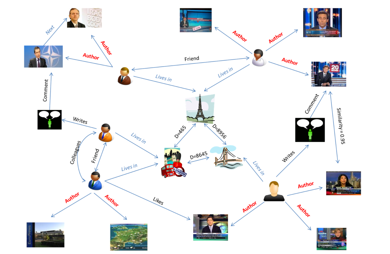
Motivation: Heterogeneous graphs

Social networks = heterogeneous nodes and relationships

Objectives

Many tasks exist

Node classification
Link prediction
Partitioning (community detection)
Collaborative Filtering
Graph classification
Information diffusion
Anomaly detection
Regression
...

Graph representation

Graph patterns
Node statistics, e.g.
- Incoming and outgoing edges
- “Distance” to other nodes
- ...

Limitations

Might not be adapted to the problem
Human expertise

Learning representations

Similarility with the problem of word representation

Objectives

Homogeneous representation space: each node $n$ corresponds to

x_n \in \mathbb{R}^n

No human expertise
Latent space geometry reflects properties of entities
Handle content (image, text, ...)

\Rightarrow

State of the art

Graphs and representations

Knowledge graphs [Jenatton 12, Bordes 13,...]
$p(x_i \rightarrow x_j) \sim \bbar z_i-z_j+z_r\bbar ^2$
Neighborhood prediction [Mikolov13,Perozzi 14,Grover 16,...]
$p(x_j|x_i) \propto \sigma(z_i \cdot z_j)$
Task specific cost
Classification
Graph Neural Networks [Scarselli 09], Embeddings [Jacob 14]
Regression
Embeddings [Ziat 15, Smirnova 16], ...
Recommendation
Matrix Factorization [Koren 09], ...
Attributed graphs: Graph CNN [Defferrad 16, Kipf 17], ...

Why uncertain representations?

Representation models should cope with:

Lack of information (= isolated nodes)
Contradictory information (= neighbors with conflicting properties)

Using distributions instead of fixed points

Mean reflects usual embedding properties
Lack of information = prior variance
Contradictory information = increases variance
Relationships

Why not Bayesian approaches?

Bayesian approach = estimate the posterior

p(\theta | \mathcal D)

\theta

= learned representations

\mathcal D

= data

Limitations

Model flexibility (interaction between linked nodes)
Learning and inference complexity

Gaussian representations

Vilnis et al. (2015): Word Representations via Gaussian Embedding

Unsupervised word representation
Skip-Gram adaptation
Gaussian densities $Z_i$ for each word $i$

-E(Z_i, Z_j) = D_{KL}(Z_i \bbar Z_j) = \int_{x \in \mathbb{R}^n} \mathcal{N}(x; \mu_j, \Sigma_j) \log \frac{ \mathcal{N}(x; \mu_j, \Sigma_j) }{ \mathcal{N}(x; \mu_i, \Sigma_i) } dx

Gaussian embeddings (1 std. dev.) for selected words (Vilnus 2015)

Outline

Node classification
Node classification with Gaussian embeddings
Recommendation with Gaussian embeddings

Heterogenous graphs: classification and regression

Context

Task: Node Classification

Data: Heterogeneous graph
Node type specific labels
A subset of labelled nodes
Task: Transduction: predict missing labels
ex. Predict photo tags, user preferences, etc.

State of the art

Content-based classification

Iterative classification [Neville 00, Belmouhcine 15]

Standard classification extended to relational data
Local classifier = node attributes + neighbor labels statistics

Label propagation

Random walks [Zhu 02, Zhou 14, Nandanwar 16]
- $\tilde y_i = \sum_{ij} p_{ij} y_j$
- No objective function
- No learning (except edge weights)
Label-based regularization [Zhou 04,Belkin 06]
$\sum_i \Delta(\tilde y_i , y_i ) + \lambda \sum_{ij} \bbar \tilde y_i - \tilde y_j \bbar ^2$

State of the arts - limitations

Limits

Heterogeneity: nodes, edges and labels
Structure: nodes of same type might be far away in the graph

Solutions

Projection to homogeneous graphs
Problem: No interaction between node of different types
Graffiti: Multi-hop random walk [Angelova 12]
- Handles different node/label types
- Two-hop random walk

Deterministic model (LaHNet)

Classification loss + graph regularization

L(z, \theta) = L_{\mathrm{classification}}(z, \theta) + L_{\mathrm{Graph}}(z)

Graph classification term $L_{\mathrm{classification}}(z,\theta) = \sum_{i\in \mathcal{N}_C} \sum_{\ell \in \mathcal{L}_{t_i}} \frac{\psi_i}{\# {\mathcal{L}_{t_i}}} \Delta_C(f(z_i; \theta_\ell), y_{i\ell})$
where $\Delta_C$ is a Hinge loss, and $f(\cdot;\theta_\ell)$ a linear classifier
Graph regularization term $L_{\mathrm{graph}}(z) = \sum_{(i,j,r)} \Phi_{ij} w_r \bbar z_i - z_j \bbar ^2$

Note:

\psi

and

\phi

are hyperparameters

Properties

Connected nodes are close in the latent space

(Indirectly) connected nodes of the same type will be classified similarly
Exploits correlations between labels of (connected) nodes of different types

Learning relation-specific weights

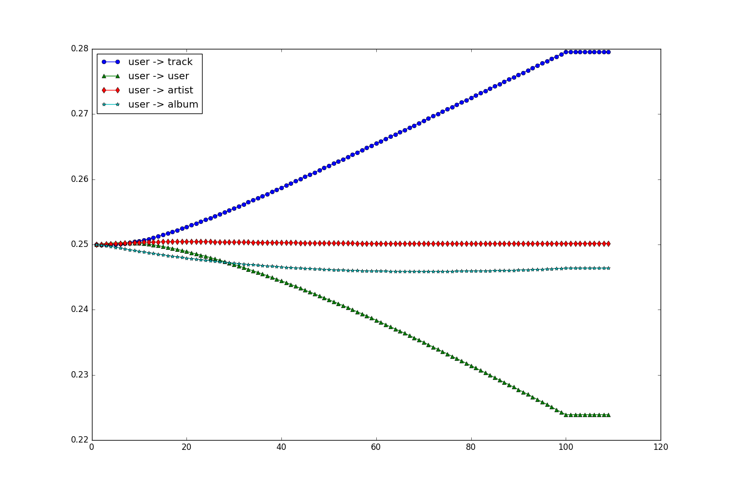
LastFM statistics

Learning relation-specific weights

Grid search: too many hyperparameters
Solution: Continous Optimization of Hyperparameter [Bengio 00, Luketina 16]
Coordinated gradient descent
- Update representations ( $z$ ) and classifiers ( $\theta$ ) with $\mathcal{N}_C$
- Update relation weights $\mathcal{N}_W$ $N_{W}$ st $\mathcal{N}_C \cap \mathcal{N}_W = \emptyset$ $N_{C} \cap N_{W} = \emptyset$ $L_W(w) = \sum_{i\in \mathcal{N}_W} \sum_{\ell \in \mathcal{L}_{t_i}} \frac{\psi_i}{\# {\mathcal{L}_{t_i}}} \Delta_C(f(z_i(w); \theta_\ell(w)), y_{i\ell})$
  Express representations wrt hyperparameters
  1. $\nabla L_{\mathrm{graph}} = 0 \implies \text{Closed form for } z_i^\star(w)$
  2. Gradient descent

Heterogeneous Classification with Gaussian Embeddings (HCGE)

Each node

i

is associated with

Z_i \sim \mathcal N(\mu_i, \Sigma_i)

where

\Sigma_i

is diagonal (D) or spherical (S)

Classification loss

(1 = 2) $\Delta_{EV}(Z, y) = \max(0; 1 - y \times \mathbb{E}_Z(f_{\theta_l}(Z))$
(1 ≠ 2) $\Delta_{Pr}(Z, y) = - \log P(y \times f_{\theta_l}(z) > 0)$

Heterogeneous Classification with Gaussian Embeddings (HCGE)

Graph Regularization loss

D_{KL}(z_j\bbar z_i) = \int_{x\in \mathbb{R}} \mathcal{N}(x; \mu_j,\Sigma_j) \log\frac{\mathcal{N}(x; \mu_j,\Sigma_j)}{\mathcal{N}(x; \mu_i,\Sigma_i)} dx

=\frac{1}{2}\left(\mathrm{tr}(\Sigma_i^{-1}\Sigma_j) + (\mu_i - \mu_j)^T\Sigma_i^{-1}(\mu_i-\mu_j) - d - \log\frac{\det(\Sigma_j)}{\det(\Sigma_i)}\right)

Experimental protocol

5 datasets (DBLP, FlickR, LastFM(x2), IMDB)
3 representative baselines
- Unsupervised (LINE)
- Homogeneous (HLP)
- Heterogeneous (Graffiti)
Evaluation = micro Precision@k
Varying size of the training set (in % of labelled nodes)

Results

Train ratio	10%			50%
Model	DBLP	Flickr	LastFM	DBLP	Flickr	LastFM
LINE	19.5	20.7	20.4	22.3	21.8	20.5
HLP	24.1	26.3	38.4	39.4	54.1	52.1
Graffiti	30.9	24.5	40.1	41.2	54.0	53.2
LaHNet	32.1	29.3	36.3	44.4	54.0	56.6
HCGE( $\Delta_{EV}$ ,S)	30.9	32.7	44.0	44.6	55.8	60.4
HCGE( $\Delta_{EV}$ ,D)	30.4	32.6	43.6	43.9	55.8	60.3
HCGE( $\Delta_{Pr}$ ,S)	27.9	29.7	27.8	45.5	54.8	58.5
HCGE( $\Delta_{Pr}$ ,D)	28.3	31.9	29.4	45.7	55.9	58.9

Learned weight

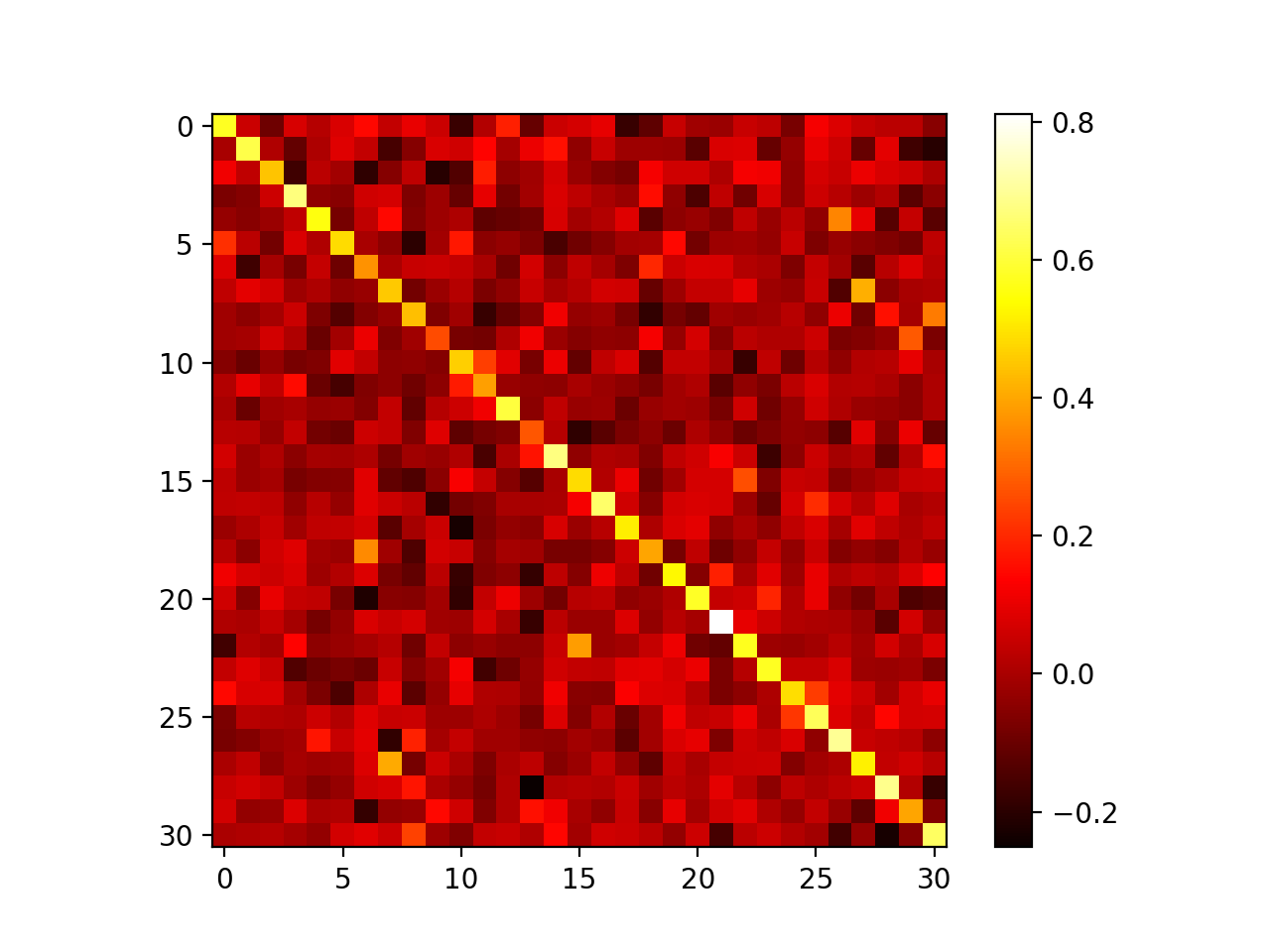
Classifiers interaction

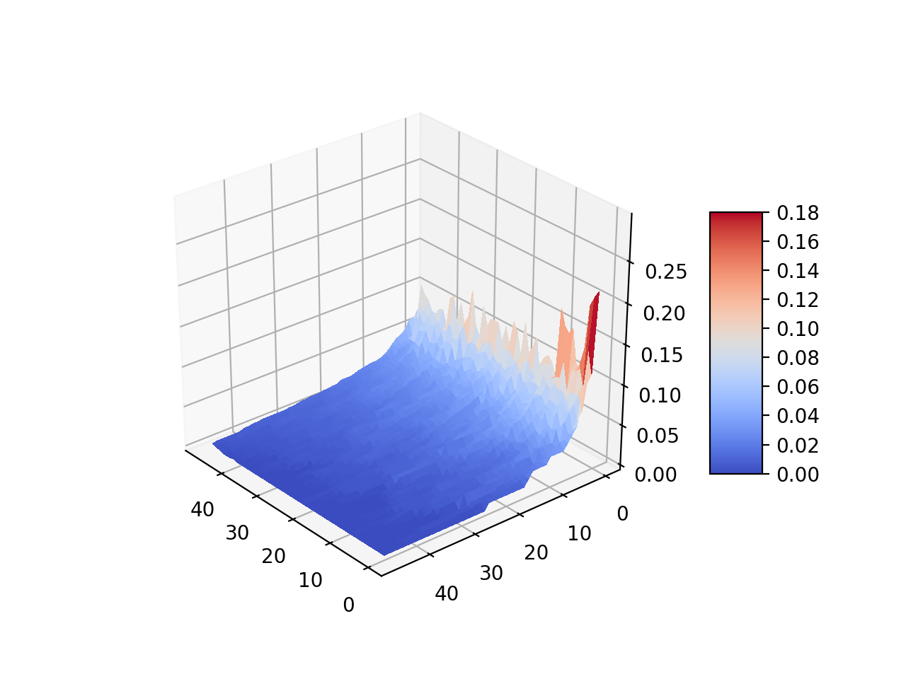
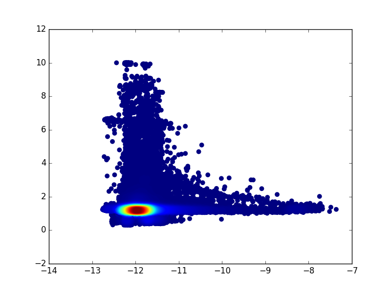
Cosine of linear classifiers parameters (LastFM) for tracks and users (common labels)

HCGE: PageRank vs Variance

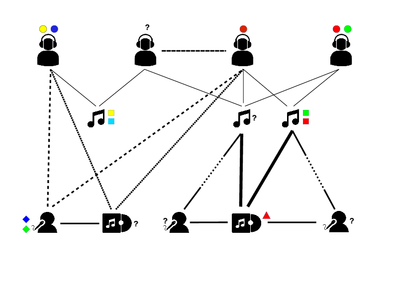
Recommendation

Task

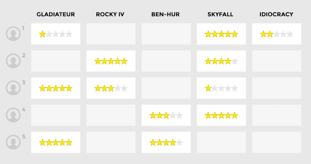
Collaborative filtering

Data = Ratings given by users on a (small) subset of items
Goal = recommend new items to users
Hypothesis = Users that rated similarly items will rate similarly new items

Matrix factorization

Koren (2009): Matrix Factorization Techniques for Recommender Systems

Score = inner product of user/item representations + bias

r_{ui} = \mu_i \cdot \mu_u + b_i

Optimized by minimizing LSE (with some regularization)

\sum_{(u,i)} \bbar \hat r_{ui} - r_{ui} \bbar ^2

Learning to rank approaches in recommendation

Pointwise

Regression: Matrix factorization (Koren 2009)
Classification: Each class is an item to recommend (Covington 2016)

Pairwise

BPR (Bayesian Personalized Ranking): likelihood of observed preferences (Rendle 2009)
Neural-network based: matching preferences (Sidana 2018)

Listwise

CliMF: reciprocical rank (Shi 2012)
CofiRank: lower bound of nDCG (Weimer 2007)

Limits

The main limits of these models

Cold-start: Usually dealt with using meta-information
Contradictions in ratings: No satisfying solution
Diversification: No direct way to estimate the covariance of results (Wang et Zhu, 2009)

Gaussian model for recommendation

X_u \sim \mathcal N(\mu_u, \Sigma_u) \text{ and } X_i \sim \mathcal N(\mu_i, \Sigma_i)

with

\Sigma_\bullet = \mathrm{diag}(\sigma_{\bullet 1}, \ldots, \sigma_{\bullet d})

Prior on (mean, precision) is a Normal-Gamma distribution (with mode: mean 0, variance 1)

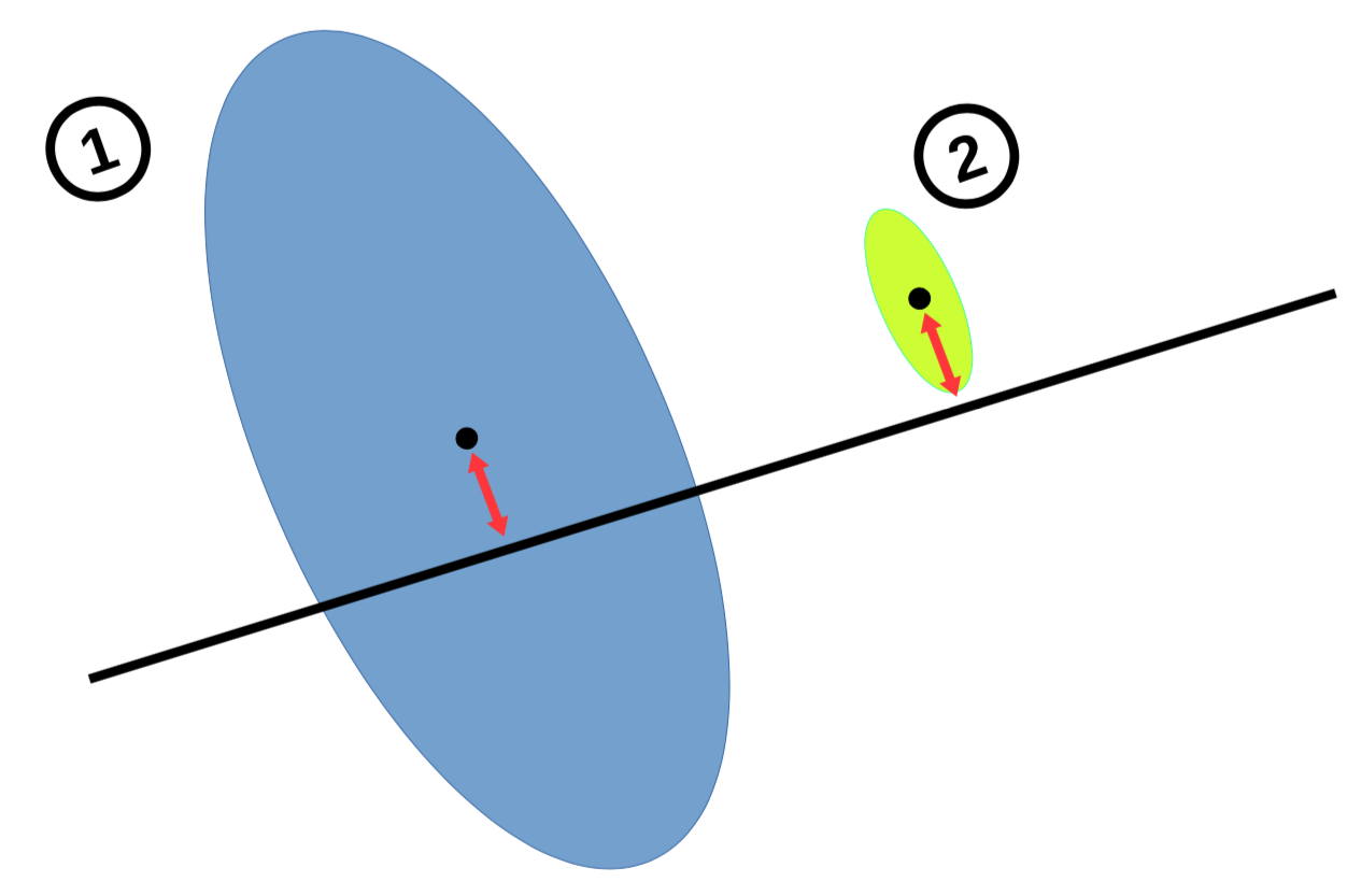
Gaussian representations

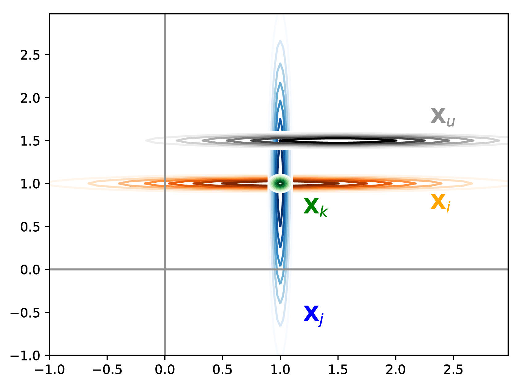
Three items having the same mean but a different variance, and a user

Pairwise learning to rank (GER-P)

Maximum A Posteriori criterion

p\left(\mathcal D|\Theta\right)p(\theta)=\prod_{\left(u,i,j\right)\in \mathcal D}p \left(i>_{u}j|\Theta\right)p(\theta)

BPR

p\left(i>_{u}j|\Theta\right)=\sigma\left(\underbrace{\mu_{i}\cdot \mu_{u} +b_i }_{r_{ui}} - \underbrace{(\mu_{j}\cdot \mu_{u}+b_j)}_{r_{uj}}\right)

GER-P

p\left(i>_{u}j|\Theta\right) = p\left(\RVX_{i}\cdot\RVX_{u}+b_{i}>\RVX_{j}\cdot\RVX_{u}+b_{j}|\Theta\right)

=p\Big(\underbrace{\RVX_{u}\cdot\left(\RVX_{j}-\RVX_{i}\right)}_{\RV{Z}_{uij}}<b_{i}-b_{j}\Big|\Theta\Big)

Pairwise learning to rank (GER-P)

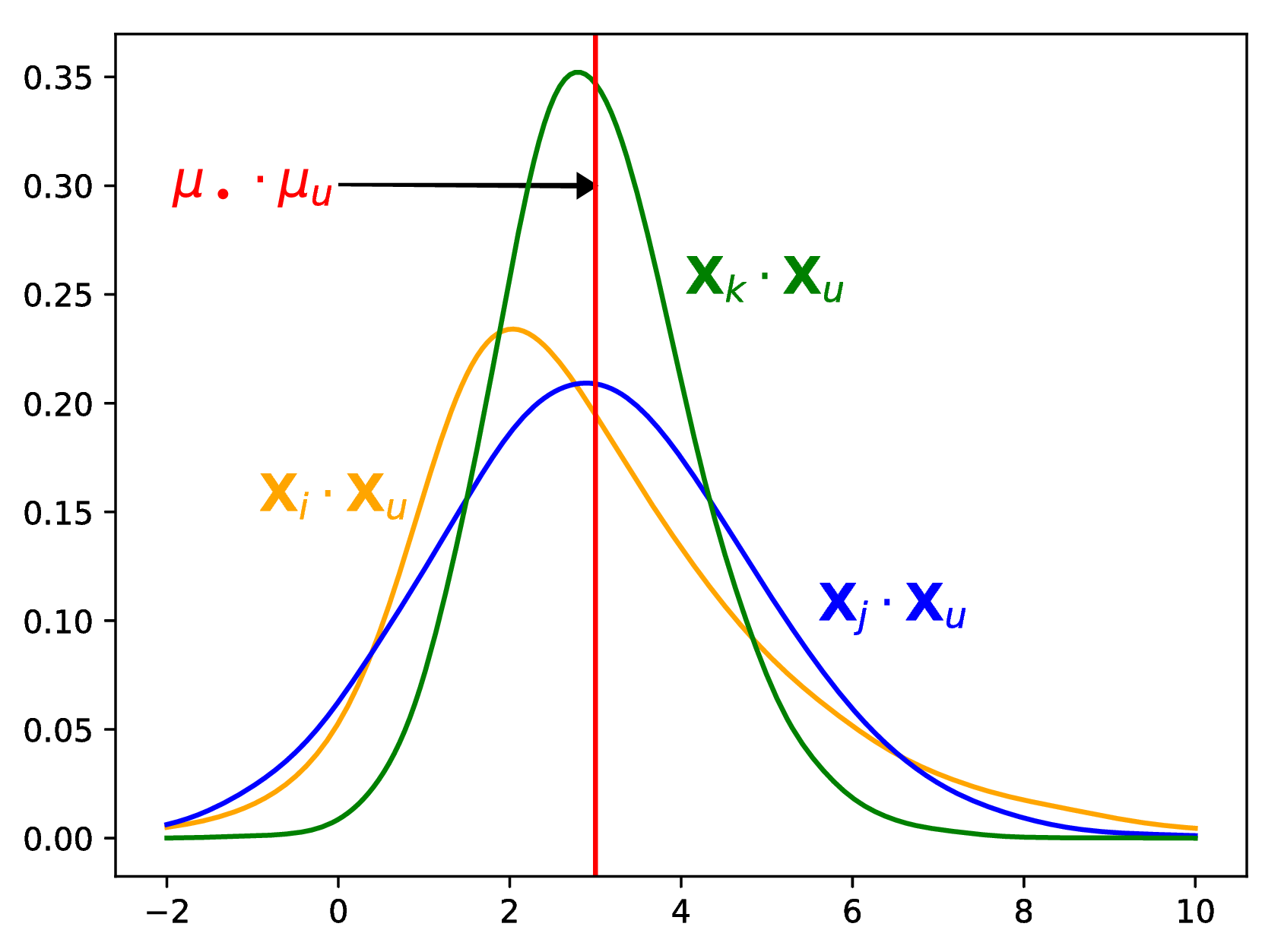
We approximate

\RV{Z}_{uij}

using a normal with matching moments:

\mathbb{E}\left[ \mathbf{Z}_{uij} \right] = \mu_u^{\top}(\mu_j - \mu_i)

\mathrm{Var}\left[\mathbf{Z}_{uij}\right] = 2\mu_u^{\top} \left(\Sigma_i + \Sigma_j\right) \mu_u + \left(\mu_j-\mu_i\right)^{\top}\Sigma_u (\mu_j-\mu_i) +\mathrm{tr}\left(\Sigma_u \left(\Sigma_j + \Sigma_i\right) \right)

Brown (1977) Means and Variances of Stochastic Vector Products with Applications to Random Linear Models

In practice, we make an error of ± 0.05 in the estimation in 99% of the samples

Listwise learning to rank (GER-L)

SoftRank

Optimizes

\mathbb{E}(nDCG | u, \RV{I}_u)

nDCG = \frac{1}{CG_{\max}} \sum_{(i,r) \in \mathrm{list}} g(i) d(r)

GER-L

p(\RV S | u, \RV{I}_u) = \mathbb{E}(nDCG | u, \RV{I}_u) = \sum_{r} \sum_{i} p(\RV{S} | r, \RV{u}, \RV{i}, \RV{I}_u) p(\RV{R} = r| \RV{u}, \RV{i}, \RV{I}_u) P(\RV{i}| \RV{u}, \RV{I}_u)

Listwise learning to rank (GER-L)

with

p(\RV{S} | r, \RV{u}, \RV{i}, \RV{I}_u) = \frac {g(i) d(r)}{CG_{\max}}

Recursion

P(\RV{R} = r | \RV{i}, \RV{I}_u \cup \{j\}) = P(\RV{R} = r | \RV{i}, \RV{I}_u) P(i >_u j) + P(\RV{R} = r - 1 | \RV{i}, \RV{I}_u) P(i <_u j)

We then use a maximum a posteriori framework (contrarily to SoftRank)

\theta^\star = \mathrm{argmax}_{\theta} \log p(\theta) + \log \underbrace{p(\RV S | u, \RV{I}_u, \theta)}_{\mathrm{observation}}

Ranking

Direct

i >_{u} j \iff p\left(i>_{u}j|\Theta\right) > 0.5

which gives

s_{ui} = \mu_u \cdot \mu_i + b_i

Positive

Exploits the variance of the score

s_{ui} = p(\RVX_u \cdot \RVX_i + b_i > 0)

Portfolio

Tries to balance risk (depending on

\alpha

)

\Exp\left({\sum_{i\in L} \RV{S}_{ui}}\right) - \alpha \Var\left(\sum_{i\in L} \RV{S}_{ui}\right)

Optimized using a greedy approach

\mathbb{E}(\RV{S}_{ui}) - \alpha V(\RV{S}_{ui}) - 2 \alpha \sum_{j \in L_n} cov\left({\RV{S}_{ui}, \RV{S}_{uj}}\right)

Experimental protocol

3 datasets (Movielens 100k, Yahoo and Yelp) for GER-P, Movielens 1M for GER-L
GER-P is evaluated with the "positive" stategy (GER-L with all)
Metric = nDCG@1, @5 and @10 (reranking of test items)
Baselines = Most Popular (MP), Soft Margin (SM), (BRPMF) BPR, CofiRank

Statistics

Dataset	Users			Items			Ratings
% Train	10	20	50	10	20	50	10	20	50
Yahoo!	3386	1645	286	1000	1000	995	159	100	33
MovieLens	743	643	448	1336	1330	1307	95	91	81
Yelp	13775	8828	3388	44877	39355	27878	980	791	467

Experimental results (GER-P / Yahoo)

Train Size $\rightarrow$	10			30			50
Model $\downarrow$	N@1	N@5	N@10	N@1	N@5	N@10	N@1	N@5	N@10
MP	53.0	59.1	67.3	52.5	58.3	66.4	53.6	57.8	64.0
BPRMF	52.8	59.0	67.2	52.2	58.3	66.4	52.2	57.7	63.5
SM	50.9	56.7	65.4	49.7	55.6	64.2	49.9	54.1	60.3
CR	53.5	60.3	68.2	57.8	61.7	68.9	56.0	60.0	65.6
GER-P	53.5	60.3	68.3	53.8	60.7	68.2	54.3	59.6	65.3

Experimental results (GER-P / MovieLens 100K)

Train Size $\rightarrow$	10			30			50
Model $\downarrow$	N@1	N@5	N@10	N@1	N@5	N@10	N@1	N@5	N@10
MP	66.0	64.7	65.8	68.4	65.3	66.3	69.1	67.4	67.5
BPRMF	66.1	64.6	65.7	66.3	64.3	65.8	66.9	65.0	66.2
SM	55.9	57.5	60.3	58.3	59.6	61.6	58.6	60.4	62.5
CR	69.0	67.3	68.6	69.7	68.5	69.5	71.4	69.4	70.6
GER-P	70.3	67.7	70.0	72.0	69.5	71.1	72.5	71.3	71.5

Experimental results (GER-P / Yelp)

Train Size $\rightarrow$	10			30			50
Model $\downarrow$	N@1	N@5	N@10	N@1	N@5	N@10	N@1	N@5	N@10
MP	40.7	41.5	46.9	39.5	39.9	44.7	37.4	37.6	41.4
BPRMF	40.8	41.3	46.8	39.6	39.8	44.6	37.3	37.2	40.9
SM	37.3	38.3	44.4	35.8	36.9	41.9	33.4	34.1	38.0
CR	47.1	46.9	51.1	46.5	46.6	50.4	46.2	45.8	48.6
GER-P	55.2	52.2	56.2	57.4	53.5	56.4	58.2	53.7	55.3

Experimental results (GER-L / MovieLens 1M)

Preliminary results

Train Size $\rightarrow$	10			30			50
Model $\downarrow$	N@1	N@5	N@10	N@1	N@5	N@10	N@1	N@5	N@10
BPRMF	56.9	54.0	54.9	57.5	54.2	54.6	55.9	53.1	53.2
BPR-L	65.5	59.7	56.8	66.0	60.5	57.0	65.9	59.4	55.6
SOFTRANK-L	64.5	59.2	57.5	66.0	60.2	56.9	65.3	59.3	55.6
GER-P	68.5	62.3	58.1	67.3	61.4	56.9	68.0	61.1	56.2
GER-L	67.2	61.5	57.8	67.3	61.7	57.3	68.4	61.7	56.5

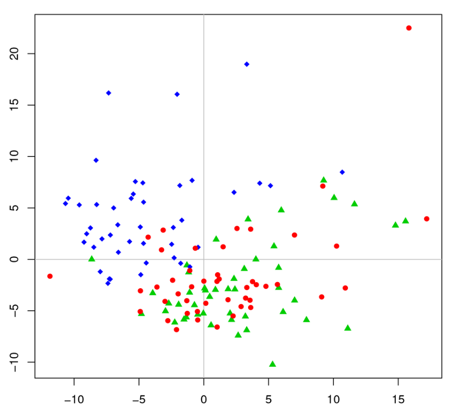
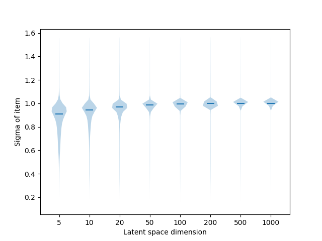
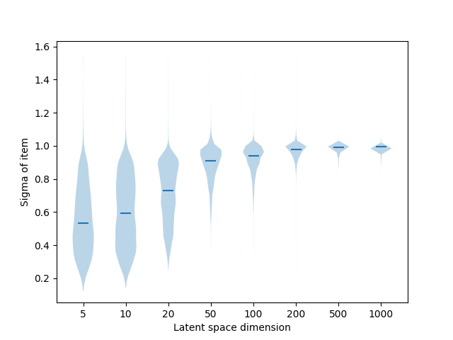
Qualitative results (mean and variance)

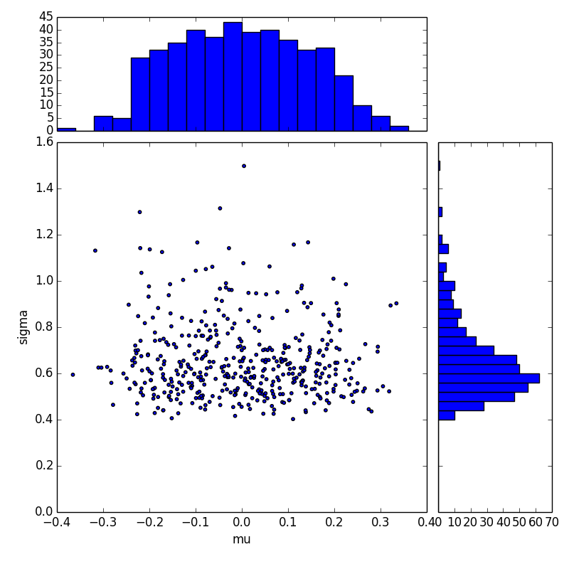
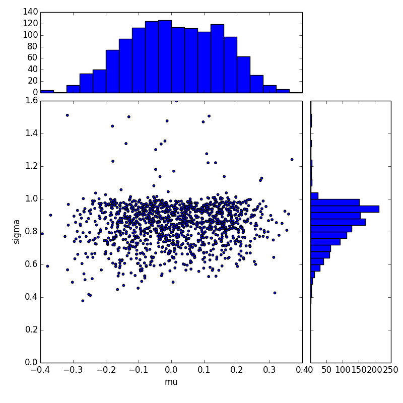
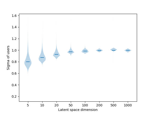
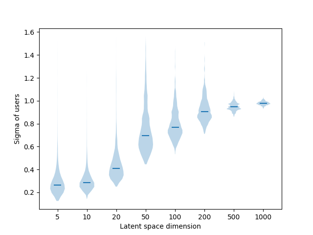
Qualitative results (variances)

Conclusion

Conclusion and ongoing work

Main points

Importance of training for the task

Representation learning for graph node classification

Importance of learning hyperparameters

Gaussian representations

Successful approach in 3 tasks (recommendation, node classification and regression)

Ongoing works (Recommendation)

Full evaluation of GER-L and ranking strategies
Content-based recommendation: content $c \rightarrow \mathcal{N}(\mu(c), \sigma(c))$

Our papers

Multilabel Classification on Heterogeneous Graphs with Gaussian Embeddings (ECML 2016)

Modeling Relational Time Series using Gaussian Embeddings (NIPS Time Series workshop 2016)

Gaussian Embeddings for Collaborative Filtering (SIGIR 2017)

Représentations Gaussiennes pour le Filtrage Collaboratif (CORIA 2018)

Representation Learning for Classification inHeterogeneous Graphs with Application to Social Networks (TKKD 2018)

Graph Embedding Day, Lyon, FranceGaussian Embeddings for Relational Data

Motivation: Heterogeneous graphs

Objectives

Graph representation

Objectives

State of the art

Why uncertain representations?

Why not Bayesian approaches?

Gaussian representations

Outline

Heterogenous graphs: classification and regression

Context

State of the art

State of the arts - limitations

Deterministic model (LaHNet)

Properties

Learning relation-specific weights

Learning relation-specific weights

Heterogeneous Classification with Gaussian Embeddings (HCGE)

Classification loss

Heterogeneous Classification with Gaussian Embeddings (HCGE)

Graph Regularization loss

Experimental protocol

Results

Learned weight

Classifiers interaction

HCGE: PageRank vs Variance

Recommendation

Task

Matrix factorization

Learning to rank approaches in recommendation

Limits

Gaussian model for recommendation

Gaussian representations

Pairwise learning to rank (GER-P)

BPR

GER-P

Pairwise learning to rank (GER-P)

Listwise learning to rank (GER-L)

SoftRank

GER-L

Listwise learning to rank (GER-L)

Ranking

Experimental protocol

Statistics

Experimental results (GER-P / Yahoo)

Experimental results (GER-P / MovieLens 100K)

Experimental results (GER-P / Yelp)

Experimental results (GER-L / MovieLens 1M)

Qualitative results (mean and variance)

Qualitative results (variances)

Conclusion

Conclusion and ongoing work

Our papers

Graph Embedding Day, Lyon, France
Gaussian Embeddings for Relational Data